Introduction To Data Structure and Algorithms
Data structure and algorihtms are two different things that play a crucial role in computer science. Data structure is defined as a particular way of storing and organizing data in our devices to use data efficiently and effectively. The main idea behind using data structures is to minimize the time and space complexities. An efficient data structure takes minimum memory space and requires minimum time to exeute the data. examples like Array , Linked list , Stack , Queue etc. An Algorithm is a step-by-step procedure or set of instructions designed to solve a particluar problem or perform a specific task
What is Time Complexity ?
How can you decide if a program written by you is efficient or not , this is measured by complexities. time complexity is used to measure the amount of time required to execute the code. time complexity is the study of efficiency of algorithm. (How much time taken to execute an algorihtm as its size grows or input size grows)
What is Space Complexity ?
It is the amount of memory or storage space required by an algorihtm to solve a computational problem as a function of the size of the input. It is a measure of how efficiently an algorithm utilizes memory resources during its execution. Both of these complexities are measured with respect to input parameter.
The Time Required for executing a code depends on serveral factors, such as :-
- The number of operation to be performed in the program
- The speed of the device and also ,
- The speed of data transfer if bieng executed on an online plateform.
What is Asymptotic Notation?
Asymptotic notation is a mathematical notation used to describe the behavior of functions as their input size increases. This does not require execution of code. the following three are notations are commonly used to represent the time complexity of algorihtm. To Compare any algorithm with another algorithm, we use these notations.
- Big-O Notations (O) :- Big-O notation describes the best and average and worst scenarios. Big-O notation is a way to express the upper bound or worst case time complexity of an algorithm. it describes the performance or efficiency of an algorithm in terms of how its running time or space requirements grow as the input size increases.
- Omega Notation :- Omega notation describes the lower bound or best-case scenarios of an algorithm's time complexity. It represents the minimum time taken by an algorithm for any input size. In other words, it provides a guarantee that the algorithm will perform at least as well as the function described by Omega notation.
- Theta Notation :- Theta notation describes both the upper bound and the lower bound, giving a tight asymptotic bound on the growth rate of the algorithm. It implies that the algorithm's runtime behaves exactly as the function described by Theta notation for sufficiently large input sizes. However, Theta notation typically represents the average-case complexity only when the best-case and worst-case complexities are the same. If the best-case and worst-case complexities differ, Theta notation usually represents the worst-case complexity.
What are Best , Worst and Average Case ?
- Best Case :- The Best case scenario for an algorithm is the situation in which it performs optimally or with minimum possible resource and time usage. For an Searching algorihtm, the best case would be when the target element is found on the first attempt and for sorting algorithm, the best case would be would be when the input data is already sorted.
- Worst Case :- The Worst case for an algorihtm is the situation in which it performs with maximum possible resources usage or it takes the most amount of time to complete. For an Searching algorihtm, the worst case occurs when the target element is at the end of the data set or not present at all. For ansorting algorithm, the worst case occurs when the input data is in reverse order.
- Average Case :- The Average case for an algorihtm consider the expected performance over all possible inputs, taking into account the likelihood of each input occurring. For an Searching algorihtm, the average case considering the probability of finding the target element at various position withing data set.
What are Upper , Lower and Tight Bound ?
- Upper Bound: it is often denoted by Big-O (O), represents the worst case scenario. Let's use a simple example to illustrate the concept of an upper bound in the context of Big-O notation. Suppose we have an algorithm that finds the maximum element in an unsorted list of numbers.
- Lower Bound :- it is often denoted by Omega, it represents the best case scenario. Let's illustrate the concept of a lower bound using same example.
- Tight Bound :- it is often denoted by theta (Θ), this provides both upper and lower limit, giving a precise description of the algorihtm growth rate. for example Θ(n) , this means the best and the worst case running time grows at the same rate as a linear function of the input size.
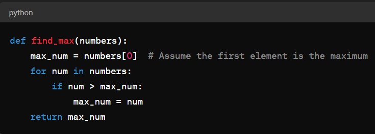
In this algorithm, as the input list numbers grows larger, the number of comparisons increases. Specifically, the algorithm compares each element of the list to the current maximum (max_num) and potentially updates max_num if it finds a larger element.
let's analyze the time complexity of this algorithm using Big-O notation.
1. Worst Case :- In the worst-case scenario, the algorihtm has to traverse through the entire list to find the maximum element. This occurs when the list is sorted in descending order or when the maximum element is at the end of the list.In this case, the algorihtm performs n - 1 comparisons, where n is the number of elements in the list.So , the time complexity of this algorihtm in the worst case is O(n) , where n is the size of the input list and O(n) is linear time which is taken by the algorihtm to run increases linearly with the size of the input.
2. Upper Bound :- the upper bound refers to the maximum amount of time an algorihtm takes to complete for any given input size. In the case of 'Find_max' algorihtm, the worst case time complexity of O(n) server as its upper bound. This means regardless of the specific input, the algorihtm will never take more then a linear amount of time to find the maximum element.
1. Best-case scenario :- If the first element in the list is the maximum, the algorihtm would only need to perform one comparison to determine that the first element is indeed the maximum. Consequently, in the best-case scenario, the algorihtm will only execute one comparison regardless of the size of the input list.
2. Lower Bound :- The Omega notation provides a lower bound on the algorihtm performance. In the best-case scenario, the algorihtm performs a constant number of comparison, Specifically one comparison. Therefore, the best case time complexity of the'Find_max' function is Ω(1). This lower bound indicates that, the algorihtm performance will not be better than constant time with respect to the size of the input ( time complexity remains constant ).
Types of Time Complexity :-
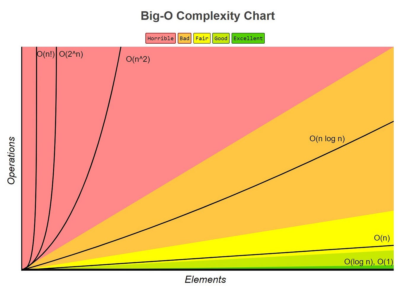
When Discussig time complexity, we often use Big O notation to express an upper bound on the growth rate of an algorihtm's runtime in terms of its input size. Big O notation provides a way to describe how the runtime of an algorihtm scales with the size of the input.
Big O notation helps us understand how an algorihtm performance will change as the input size increases and allows us to comapre the efficiency of different algorihtms. (Note :- 'n' represents the size of the input)
Types of Complexities :-
- O(1) - Constant time complexity :- This means that the runtime of the algorihtm remains constant regardless of the size of the input or no matter how big input gets, the time it takes for the algorihtm to run stays the same. for example :-
- O(Log n) : Logarithmic Time Complexity :-In this case, as the size of the input grows, the time it takes for the algorihtm to run increases , but not proportionally. In Logarithmic time complexity (O(log n)), as the size of the input (n) increases, the time taken by the algorihtm to run increases,but it des so very slowly compared to linear time complexity (O(n)).
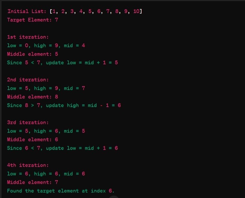
It increases slowly because the algorihtm divides the problem into smaller pieces in each step, reducing the size of the problem dramatically with each iteration. A classic example of an algorihtm wiht with Logarithmic time complexity is binary search.
In Binary Search, you have a sorted list of elements , the algorihtm repeatedly divides the search interval in half unitl the target element is found or the search interval becomes empty. Let's see its working :-- Initialize : Start with a sorted list of elements. Set two pointers 'low' and 'high', initially pointing to the first and last element of the list.
- Middle Element : Find the middle element of the current search interval by calculation 'mid = (low + high) / 2'
- Check Middle Element : Compare the middle element with the target element your're Searching for, if the middle element is equal to the target value,the search is successfull, and you can return the index of the middle element but if the middle element is greater than the target element, then we discard the upper half, including the middle element and search for the target value in lower half and if the target value is smaller than the middle element than we discard the lower half including middle element and search for the target value in the upper half.
- Repeat and Finalize : Continue the process until the key id found or the total search space is exhausted. if the target element is found, return its index and if not found then return asignal indicating its absence and end the algorihtm.
- O(n) : Linear Time Complexity :- In this, the time taken by the algorihtm to run increases linearly with the size of the input. if the input size doubles, the time taken to execute the algorihtm also doubles. Suppose you have an algorihtm that needs to search for a specific value in the unsorted list of number. In this case, the algorihtm needs to go through each element in the list to find the target value or reach the end of the list.
- O(n log n) : Linearithmic Time Complexity :- This is a bit faster then the Quadratic time. it's like having a linear time operation inside a loop that runs log n time. for larger inputs, the time increases but not as much as Quadratic time. this complexity is often seen in algorihtm that involve sorting or divide-and-conquer approaches. This time complexity indicates that the algorihtm running time grows in proportion to n multiplied by the logarithm of n. An example of of an algorihtm with O(n log n) time complexity is the Merge Sort Algorithm
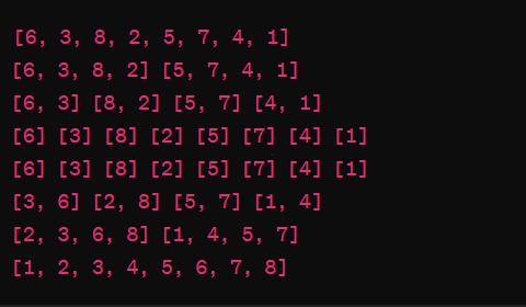
Merge Sort is a popular comparison based sorting algorihtm that follows the divide-and-conquer approach. Let's see its working : - Divide :- Divide the Unsorted list into two halves recursively unitl each sublist contains only one element.
- Conquer :- Merge the sublist back together in a sorted order.
- Combine :- As merging the sublist takes linear time, but this operation is performed log n times due to recursive nature by the algorihtm.
- O(n^2) : Quadratic Time Complexity :- In this Complexity, it is an algorihtm whose execution time grows Quadratically with the size of the input. "2" indicates that the time complexity grows proportionally to the square of the input size. for example if you have "n" elements in the input, the algorihtm might take roughly "n^2" steps to complete and if you double the size of the input from "n" to "2n", the algorihtm might take roughly four times as long to run (since (2n)^2 = 4n^2).
Bubble Sort Algorithm is the best example of this complexity. Bubble sort algorihtm is a simple sorting algorihtm that repeatedly iterates through the list, compare adjacent elements, and swap them if they are in wrong order. this is the worst-case scenario because this algorihtm will need to perform n iterations for each of the n elements in the list, resulting n * n comparison or swap.
For Example, if you have an unsorted list of 4 elements , the bubble sort may need to perform full comparsions First pass: 3 comparisons, Second pass: 2 comparisons, Third pass: 1 comparison. Each pass involves iterating through the last one and comparing adjacent elements. - O(n^3) : Cubic Time Complexity :- Similar to Quadratic time but even slower, the time it takes for the algorihtm to run increase cubically with the size of the input. if you double the size of the input from "n" to "2n", the algorihtm might take roughly four times as long to run (since (2n)^3 = 8n^3). This is used inMatrix Multiplication.
- O(2^n) : Exponential Time Complexity :- This is even much slower then previous complexity. the time it takes for the algorihtm to run grows exponentially with the size of the input. Example Recursive Algorihtm, In this given a set wiht n elements, the goal is to generate all possibel subsets of this set, including empty set and the set itself.
- O(n!) : Factorial Time Complexity :- This Complexity is the slowest of them all, the time it takes for the algorihtm to run increases factorially with the size of the input. Example Brute Force Method
_complexity.jpeg)
In this algorihtm, regardless of the size of the array 'arr, the operation of printing the first element ('arr[0]') takes a constant amount of time. Whether the array has 5 elements or 10,000 elements, the time it takes to print first element remains the same. Therefore, the time complexity of this algorihtm is O(1).