Introduction To Neural Network

Algorithm inspired by the neurons of the human brains just like neurons make up the brain , the fundamanetal building blocks of a neural network is also a neuron. Neural networks are used to recognize patterns, make predictions, and perform tasks that typically require human-like intelligence.

Neuron:-A thing that holds the number specifically between 0(for black pixels) and 1(for white pixels) like 0.8 or 0.3, no more then 1.

For Example:-The Network starts with a bunch of neurons corresponding to each pixel in a 28x28 input image which is 784 neurons in total, each one of these holds a number that represents the grayscale value of the correspondin ranging from 0 for black pixels up to 1 for white pixels. these numbers inside the neuron is called itActivation.each neuron lit up when its activation is a higher number or has passed through a threshold value like 0.58. All of these neurons(784) make up the first layer of our network.

In image processing tasks, each pixel value can be treated as a feature, and our neural network learns from these features and make predictions or perform tasks such as object detection or image classification.

The activation in these neurons ranging between 0 and 1 represents how much the system thinks that a given image corresponds wiht a given digit. the way the network operates activation in one layer determine the activation of the next layer.

If you feed an image to the network, lighting up all the 784 neurons of the input layer, according to the the brightness of each pixel in the image in the image, that pattern of activation causes some very specific pattern in the next layer, which causes some pattern in the one after it, which finally gives some pattern in the output layer and the brightest neuron of that output layer is the network choice.

Properties of neural network :-

• take in data as input.
• train themseleves to understand patterns in the data.
• predict outputs for a new set of similar data.

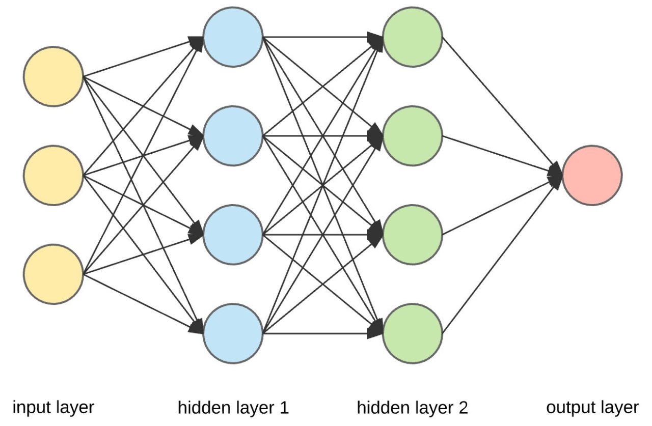
In a neural network information propagates through central components that form the base of every neural network architecture.

• Input Layer


• Hidden Layer


• Output Layer

The Learning process of a neural network can be broken into two main processes:- Forward Propagation and Backward Propagation.

Forward Propagation :-

Forward propagation is the propagation of information from the input layer to the output layer. we can define our input layer as several neurons x1 , x2 and so on. these neuron connects to the neurons of the next layer through channel and they are assigned numerical values calledweights

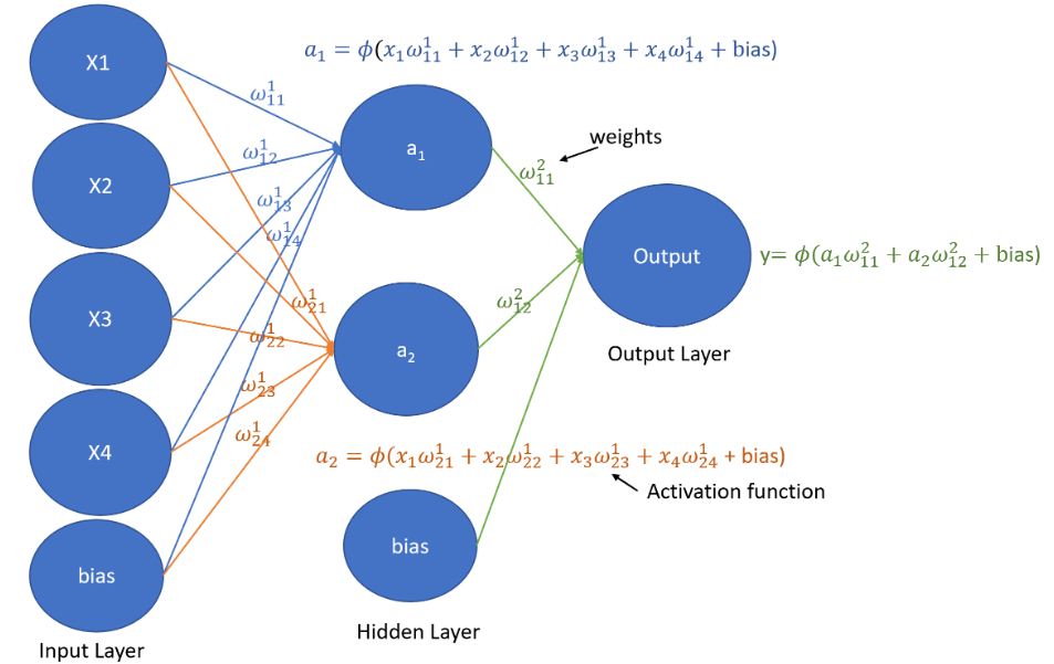
The Input (x1) are multiplied by the weights (w1), and their sum is computed. This sum is then sent as input to the neurons in the hidden layer. Each neuron in the hidden layer is associated with a numerical value called a bias, which is added to the input sum. The resulting weighted sum, now including the bias, is then passed through a non-linear function called the activation function.The activation function determines whether and to what extent that particular neuron contributes to the next layer of the neural network.

In the output layer, the neurons produce outputs on the form of probabilities using an activation function, such as softmax. Each neuron output represents the probability of a specifiv className. The neuron with the highest probability determines the final output or prediction of the neural network.

weight(w1) :-The weight of a neuron tell us how important he neuron is , the higher ther value the more important it is in the relationship.

Bias :-Is an additional parameter that is added to the input layer of each activation function. The purpose of bias is to shift the activation function to the right ot left. When bias is added, it allows the activation function to be more flexible and capable of finding complex patterns in the data.

Backward Propagation

Is almost like forward propagation except in the reverse direction. Information here is passed from the output layer to the hidden layer.

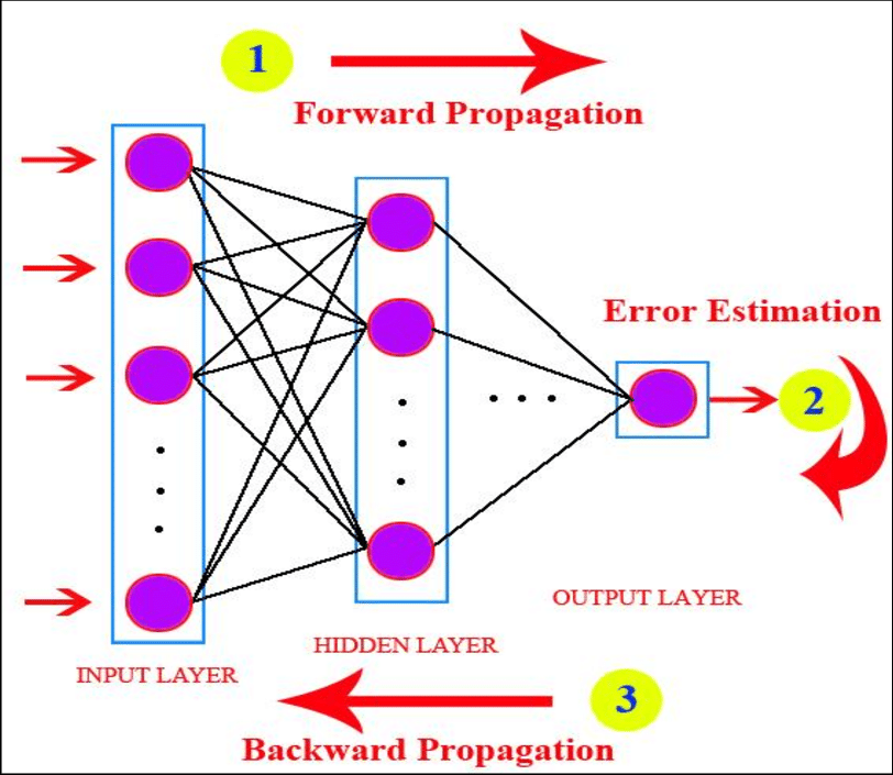
Backward propagation is the reason why neural network is so powerfull. It is the reason why neural network can learn by themseleves. In the last step before propagation, a neural network spits a prediction, this prediction could have two possibility either right ot wrong.

In Backward propagation, the neural network evaluates its own performance and checks if it is right or wrong. if it is wrongthe network uses something called the loss functionto quantify the deviation from the expected output ( the output of the neural network is compared to the actual target values using the loss function) and it is this information that is sent back to the hidden layer for the bias and weights to be adjusted, so that the network accuracy level increases.

The Learning Algorithm can be summarized as follows :-

• First Initialize parameters(bias and weights) with random values for the network parameter.


• We take a set of input data amd pass them through the neural network, we compare the predicted values which were produced by the neural network with the expected value and calculate the loss using the loss function.


• Apply Backpropagation to minimize the loss by adjusting the weights and bias through the use of the gradient descent algorithm.The objective is to iteratively reduce the total loss, leading to the improvement of the model.

Terminologies :-

• Activation Function :-Introduces non-linearity in the network and decide whether a neuron can contribute to the next layer or not. To make this decision, different activation functions are used.
  
  
  • Step function :-The First idea we had was about how we activate a neuron if it is above a certain value or threshold value, if it is less then the threshold value it won't we activated. For example:- If value more then 0 activate, else do not activate. If the input is greater then or equal to a certain threshold value(usually 0) then the output is set to one (or sometimes +1). if the input is less then the threshold value then the output is set to zero(or sometimes -1).The Step function only gives output in binary form.
  
  
  • Limitations :-
    It is not a continous function, which means that it is not differentiable at the point x = 0(input = 0). This can make it difficult to train neural network and it gives output in binary form which means that it cannot be used for tasks that require multi-value output (75%).
  
  
  • Examples of how step functions can be used in activation function :-
    
    • A Binary classifier for classifying images of cats and dogs.
    • In Logic gates, such as AND,OR and NOT.
  
  
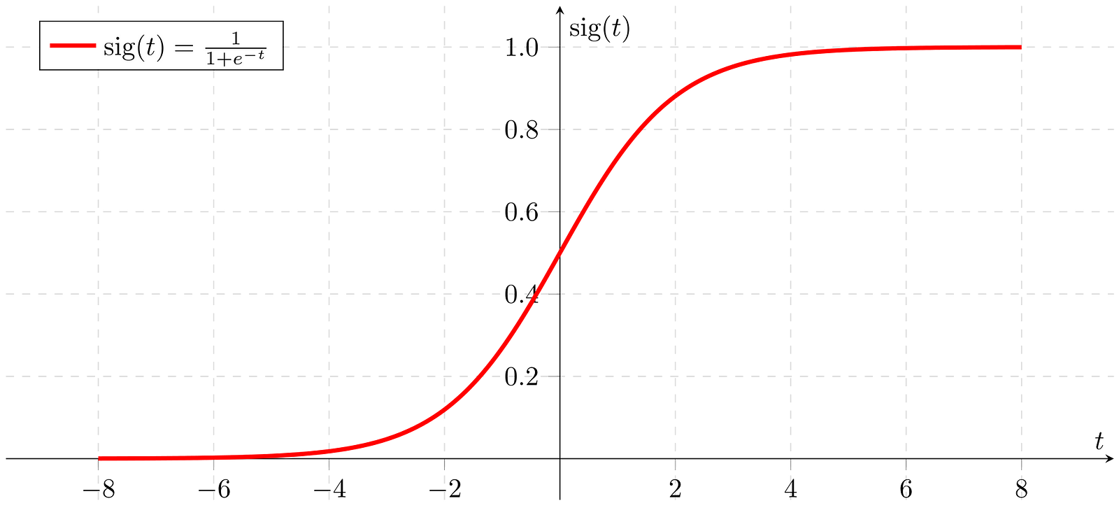
  • Sigmoid function :-The Sigmoid function is represented or define as sig(t) = 1 / (1 + e ^-t). It is non-linear which means it can learn complex relationship between data points, its range(or ouput value) is between 0 and 1 which makes it easy to interpret as a probability. It is most widely used activation functions. The sigmoid functions is a good choice for an activation function because it non-linear and differentiable.
  
  
  • The Sigmoid function is commonly applied ot the weighted sum of inputs in the neural networks.
    
    We have inputs x1,x2,x3,.....,xn and weights w1,w2,w3,....wn, the weighted sum tis calculated.
    t = w1.x1 + w2.x2 + ... + wn.xn
    
    The sigmoid function is applied to this weighted sum to squash it into the range between 0 and 1.
  
  
  
  • Limitations :-
    
    • It gives rise to the vanishing gradient problem , during back propagation, gradients(bias and weights) can become very small as they are multiplied through many layers, making it challenging for the model to learn from certain inputs.
    
    
    • Computationally Expensive.
  
  
  • Example :-
    
    • A Binary classifier for classifying images of cats and dogs.
    • A neural network for predicting the probability of a customer churning.
  
  
  • ReLu function (Reactified linear unit) :-ReLu is defined as f(x) = max(0,x). It outputs the input value if its positive and zero otherwise. The output of ReLu is in the range (0,∞). Relu functions is used as an activation function in neural network to introduce non-linearity into the model which helps model to learn complex relationship between datapoints.
  
  
  • Limitations :-
    • ReLu is a good default choice and is often used in many architecture. However, be aware of dying ReLu problem, where neuron can get stuck and always outputs zero for all inputs.
    
    
    • Exploading gradient problem during training where outputs values becomes very large or gradients becomes very large causing instability in the model.


• Loss Function :-In Learning process of neural networks we start with random weights and bias, the neural network makes a prediction, this prediction ic compared against the expected output and weights and bias are adjusted accordingly. Loss function is the reason we are able to calculate that difference. A loss function is the way to quantify the deviation of the predicted output by the neural network to the expected output.


• Optimizers :-loss function are mathematical ways of measuring how wrong prediction made by the neural network are. During the training process, we adjust the parameter (weights and bias) to make our predictions as coorect as optimized as possible. when we say "optimized", it mean that the neural network has learned a set of parameters that minimizes the error.
  
  In Simple terms, Optimizers shape and mold our model into more accurate model by adjusting the parameters and loss function is its guide, it tells the Optimizers whether it's moving in the right or wrong direction.
  
  It's impossible to know what your model weights should be right from the start but with some trial and error based on the loss function, you could end up getting there in the end.

What is Gradient Descent

Gradient descent is a method used by optimization algorithm like stochastic gradient descent. The primary goal of this is to minimize the loss function or cost function. This funtions measures the difference between the predicted value of a model and the targeted value for a given input and based on this difference we adjust our model parameters until the loss function becomes low as possible.

The process of optimizing a machine learning model using gradient descent involves calculating the difference between the actual and predicted values, then adjusting the weights of the neurons in the network based on this difference.

Working :-

1. First we calculate what a small change in each individual weights would do to the loss function.

2. Adjust each parameter based on its gradient.

3. Repeat step 1 and 2 until the loss function is as low as possible.+

Stochastic Gradient Descent :-

In standard gradient descent, the algorithm computes the gradient of the entire dataset loss function with respect to the model parameters at each iterations. it uses the complete dataset to update the parameters. But in stochastic gradient descent, it randomly selects a small subset of dataset or uses subset of traning ecamples rather then the entire dataset because of this it is less Computationally expensive.

Advantages :-

1. Faster compared to batch gradient descent and standard gradient descent, because it updates model parameters more frequently and gives good solution in few iterations.

2. SGD is more Suitable for large datasets since it process only a small portion or subset of the whole dataset reducing the memory and Computational requirements.

Disadvantages :-

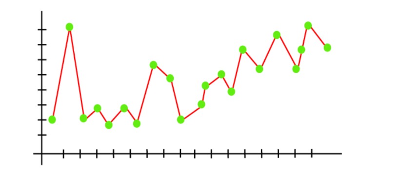
Due to its stochastic nature SGD converges more quickly then others in processing time because of each update is based on a single randomly selected data point, the parameters updated in SGD can be noisy and exhibit high variance(Overfitting).

Due to this noisy updates, the loss function may not decrease smoothly in SGD. In the image below the SGD has taken a noisy path to the target.

Paths taken by both the gradients.

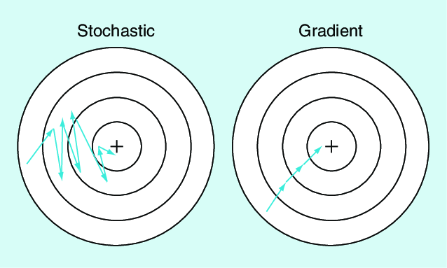
Batch Gradient Descent :-

Batch gradient descent is a variant of the gradient descent optimization algorithm where it computes the entire dataset at each iteration as a result it is very slow on a very large training data. batch gradient is more accurate but slow, while stochastic gradient is faster but less accurate as you can see in the above diagram.

Mini-Batch Gradient Descent :-

Mini-Batch gradient descent is a variant of the gradient descent optimization algorithm. it is designed to improve the efficiency of the training process, especially when dealing wiht large dataset. Improved upon batch gradient descent, it divides the training dataset into smaller, random subsets called mini-batches.

Instead of computing the gradient using the entire dataset, A mini-batch of data is used in each iteration.

Regularization :-

The Central problem in deep learning is how to make an algorihtm that will perform well not just in training dataset but also in the new dataset or new input. The most common challenges faced when you will training the model is Overfitting.

Overfittingis a problem or a situation where your model perform exceptionally well on training dataset but not in testing dataset.

Regularizationare techniques that are used to prevent or reduce overfitting in the model and improve the generalization performance of a neural network.

Types of Regularization :-

1. Dropout :-It produces very good results and is consequently , the most used regularization technique in the field. We will understand dropout with the help of an example, let's say we have a neural network with two hiddent layers, what dropout does is at every iteration, it randomly selects some nodes and drop or remove them along with incoming and outgoing connection.

Because of this the model will memorize less the training data, hence will genralize better and build a more robust prediction model.

2. L1 Regularization (Lasso) :-Let's understand this with an example, Imagine you are building a model with many features and L1 regularization encourages the model to only learn a subset of the most important features by adding a penalty for having too many non-zero weights. It shrinks some weights to exactly zero and removing some features from the model.

3. L2 Regularization (Ridge) :-Also prevents overfitting, but in a different way, it discourages any single weight from becoming extremely large by adding a penalty for having large weight.

It encourages all weights to to be small and preventing them from becoming too big, which helps in avoiding overfitting and relying too heavly on just one feature or few features.

4. Data Augmentation :-Sometimes the best way to make deep learning model genralize better is to train it on more data. we have a limited set of data and one way to get this problem solved by generating additional training samples or examples by applying random transformations to existing data, such as rotation, zooming, flipping etc.

5. Early Stopping :-In this, we monitor the performance of the model on a validation dataset during training and stops the training process when the performance starts to digrade this helps prevent the model from overfitting the trainig dataset.

6. Batch Normalization :-This hepls stabilize the training process by normalizing the input of each layer during training which leads to faster convergence and better generalization.

Feed Forward Neural Network (FFN) :-

It is type of neural network architecture that consists of multiple layers of neurons, where each neuron in a layer is connected to every neuron in next layer with no-backward connections, no-cycles or loops in the connection of the network.

Neurons have activation functions like linear , sigmoid , ReLu , etc. Each type of activation function has its prons and cons, so we use them in various layer in deep neural network.

Inputs , Outputs , Hidden Layers(Hidden Units), Neurons per hidden layer , Activation function , Forward propagation , loss function , Back-propagation and optimization process. These numerous combination allow is to create a variety of powerful deep neural networks that can solve complex problems by learning patterns within data.

The more neurons we add to the hidden layer, the wider the network becomes.